Bayesian performance analysis example in pyfolio

There are a few advanced analysis methods in pyfolio based on Bayesian statistics.

The main benefit of these methods is uncertainty quantification. All the traditional measures of performance, like the Sharpe ratio, are just single numbers. These estimates are noisy because they have been computed over a limited number of data points. So how much can you trust these numbers? You don't know because there is no sense of uncertainty. That is where Bayesian statistics helps as instead of single values, we are dealing with probability distributions that assign degrees of belief to all possible parameter values.

Lets create the Bayesian tear sheet. Under the hood this is running MCMC sampling in PyMC3 to estimate the posteriors which can take quite a while (that's the reason why we don't generate this by default in create_full_tear_sheet).

Import pyfolio

%matplotlib inline
import pyfolio as pf

Fetch the daily returns for a stock

stock_rets = pf.utils.get_symbol_rets('FB')

Create Bayesian tear sheet

out_of_sample = stock_rets.index[-40]

pf.create_bayesian_tear_sheet(stock_rets, live_start_date=out_of_sample)

Running T model


WARNING (theano.gof.compilelock): Overriding existing lock by dead process '23486' (I am process '24728')


Applied log-transform to volatility and added transformed volatility_log to model.
Applied log-transform to nu_minus_two and added transformed nu_minus_two_log to model.
 [-----------------100%-----------------] 2000 of 2000 complete in 14.8 sec
Finished T model (required 279.00 seconds).

Running BEST model
Applied interval-transform to group1_std and added transformed group1_std_interval to model.
Applied interval-transform to group2_std and added transformed group2_std_interval to model.
Applied log-transform to nu_minus_two and added transformed nu_minus_two_log to model.
 [-----------------100%-----------------] 2000 of 2000 complete in 12.6 sec
Finished BEST model (required 132.06 seconds).

Finished plotting Bayesian cone (required 0.21 seconds).


/home/wiecki/miniconda3/lib/python3.5/site-packages/matplotlib/axes/_axes.py:519: UserWarning: No labelled objects found. Use label='...' kwarg on individual plots.
  warnings.warn("No labelled objects found. "



Finished plotting BEST results (required 1.45 seconds).

Finished computing Bayesian predictions (required 0.26 seconds).

Finished plotting Bayesian VaRs estimate (required 0.12 seconds).

Running alpha beta model
Applied log-transform to sigma and added transformed sigma_log to model.
Applied log-transform to nu_minus_two and added transformed nu_minus_two_log to model.
 [-----------------100%-----------------] 2000 of 2000 complete in 7.2 sec
Finished running alpha beta model (required 130.28 seconds).

Finished plotting alpha beta model (required 0.24 seconds).

Total runtime was 543.62 seconds.

Lets go through these row by row:

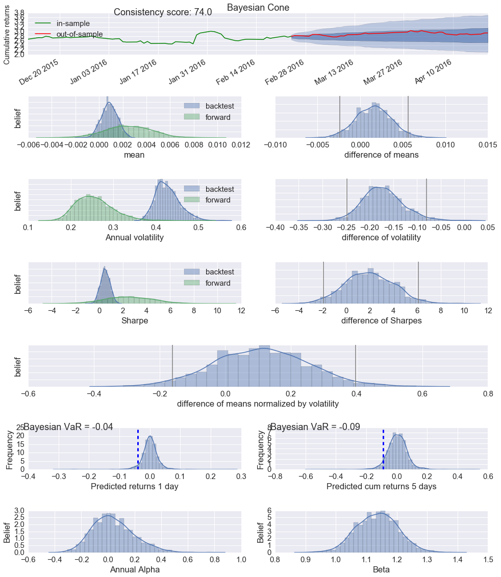
• The first one is the Bayesian cone plot that is the result of a summer internship project of Sepideh Sadeghi here at Quantopian. It's similar to the cone plot you already saw in the tear sheet above but has two critical additions: (i) it takes uncertainty into account (i.e. a short backtest length will result in a wider cone), and (ii) it does not assume normality of returns but instead uses a Student-T distribution with heavier tails.
• The next row compares mean returns of the in-sample (backest) and out-of-sample or OOS (forward) period. As you can see, mean returns are not a single number but a (posterior) distribution that gives us an indication of how certain we can be in our estimates. The green distribution on the left side is much wider, representing our increased uncertainty due to having less OOS data. We can then calculate the difference between these two distributions as shown on the right side. The grey lines denote the 2.5% and 97.5% percentiles. Intuitively, if the right grey line is lower than 0 you can say that with probability > 97.5% the OOS mean returns are below what is suggested by the backtest. The model used here is called BEST and was developed by John Kruschke.
• The next couple of rows follow the same pattern but are an estimate of annual volatility, Sharpe ratio and their respective differences.
• The 5th row shows the effect size or the difference of means normalized by the standard deviation and gives you a general sense how far apart the two distributions are. Intuitively, even if the means are significantly different, it may not be very meaningful if the standard deviation is huge amounting to a tiny difference of the two returns distributions.
• The 6th row shows predicted returns (based on the backtest) for tomorrow, and 5 days from now. The blue line indicates the probability of losing more than 5% of your portfolio value and can be interpeted as a Bayesian VaR estimate.
• The 7th row shows a Bayesian estimate of annual alpha and beta. In addition to uncertainty estimates, this model, like all above ones, assumes returns to be T-distributed which leads to more robust estimates than a standard linear regression would. The default benchmark is the S&P500. Alternatively, users may use the Fama-French model as a bunchmark by setting benchmark_rets="Fama-French".
• By default, stoch_vol=False because running the stochastic volatility model is computationally expensive.
• Only the most recent 400 days of returns are used when computing the stochastic volatility model. This is to minimize computational time.

Running models directly

You can also run individual models. All models can be found in pyfolio.bayesian and run via the run_model function.

help(pf.bayesian.run_model)

Help on function run_model in module pyfolio.bayesian:

run_model(model, returns_train, returns_test=None, bmark=None, samples=500, ppc=False)
    Run one of the Bayesian models.

    Parameters
    ----------
    model : {'alpha_beta', 't', 'normal', 'best'}
        Which model to run
    returns_train : pd.Series
        Timeseries of simple returns
    returns_test : pd.Series (optional)
        Out-of-sample returns. Datetimes in returns_test will be added to
        returns_train as missing values and predictions will be generated
        for them.
    bmark : pd.Series or pd.DataFrame (optional)
        Only used for alpha_beta to estimate regression coefficients.
        If bmark has more recent returns than returns_train, these dates
        will be treated as missing values and predictions will be
        generated for them taking market correlations into account.
    samples : int (optional)
        Number of posterior samples to draw.
    ppc : boolean (optional)
        Whether to run a posterior predictive check. Will generate
        samples of length returns_test.  Returns a second argument
        that contains the PPC of shape samples x len(returns_test).

    Returns
    -------
    trace : pymc3.sampling.BaseTrace object
        A PyMC3 trace object that contains samples for each parameter
        of the posterior.

    ppc : numpy.array (if ppc==True)
       PPC of shape samples x len(returns_test).

For example, to run a model that assumes returns to be normally distributed, you can call:

# Run model that assumes returns to be T-distributed
trace = pf.bayesian.run_model('t', stock_rets)

Applied log-transform to volatility and added transformed volatility_log to model.
Applied log-transform to nu_minus_two and added transformed nu_minus_two_log to model.
 [-----------------100%-----------------] 500 of 500 complete in 1.9 sec

The returned trace object can be directly inquired. For example might we ask what the probability of the Sharpe ratio being larger than 0 is by checking what percentage of posterior samples of the Sharpe ratio are > 0:

# Check what frequency of samples from the sharpe posterior are above 0.
print('Probability of Sharpe ratio > 0 = {:3}%'.format((trace['sharpe'] > 0).mean() * 100))

Probability of Sharpe ratio > 0 = 92.0%

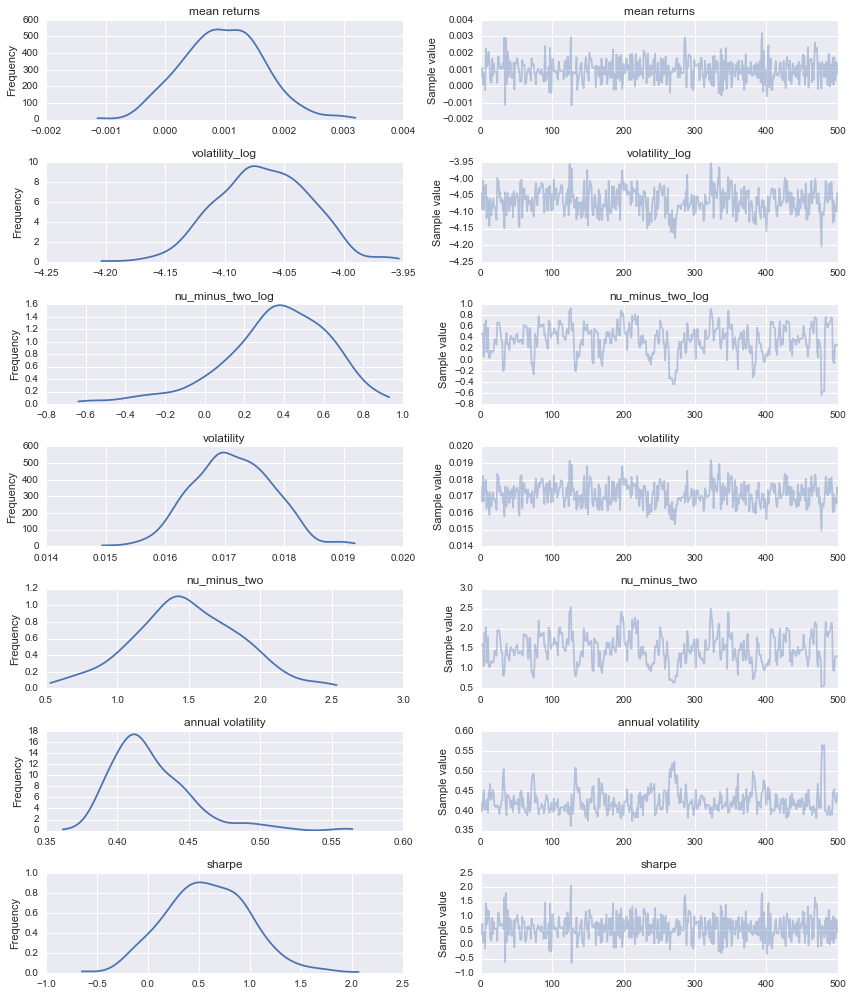
But we can also interact with it like with any other pymc3 trace:

import pymc3 as pm
pm.traceplot(trace);

Further reading

For more information on Bayesian statistics, check out these resources:

• A blog post about the Bayesian models with Sepideh Sadeghi
• My personal blog on Bayesian modeling
• A talk I gave in Singapore on Probabilistic Programming in Quantitative Finance
• A series of IPython notebooks on Bayesian Methods for Hackers.